CUDA 101: Matrix-Vector Product
The foundation of GPU programming is linear algebra. This post takes you from a basic linear algebra example problem to a GPU-accelerated example that calculates a matrix-vector product.
These views do not in any way represent those of NVIDIA or any other organization or institution that I am professionally associated with. These views are entirely my own.Key Takeaways
- Correctness precedes parallelism and performance
- Identify and understand the underlying algorithms at play
- Speed is not the same as efficiency
- Use sane defaults, only optimize after profiling and testing
- Use the most specialized tool for the job
NOTE: This post is geared towards those without significant experience in linear algebra, high performance computing, or GPU programming.
Outline
- Mathematical Understanding of Algorithm
- Algorithm Analysis
- C on the Host
- CUDA C
- Core Concepts
- Host and Device
- Using the CUDA Runtime
- Shared Memory
- CUDA Mat-Vec Multiply
- Core Concepts
- CUDA C++
- Naive Approach
- More Sophisticated Approach
- The Best Tool for the Job
- Conclusion
- BQN Example
- Links, References, Additional Reading
Mathematical Understanding of Algorithm
We’ll be performing a matrix-vector dot product several ways in this post.
The operation is depicted below:
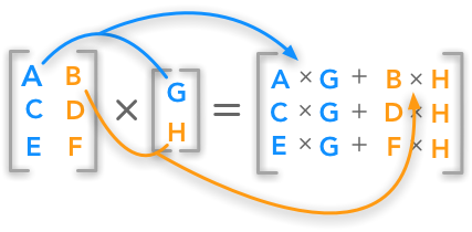
Let p be the result of the dot product of matrix Mat and vector v.
The dot product is calculated like so:
Notice how values of v are broadcast to match the shape of Mat:
We can broadcast values of v into columns of a matrix with the same shape as the matrix Mat, and then pair the Mat and v element-wise, creating a matrix of tuples (or a 3d matrix if you prefer):
This is sometimes called a tuple space, or the domain of our algorithm. The book How to Write Parallel Programs: A First Course covers tuple spaces in great detail.
Now that we have constructed our tuple space, we might group our computations into self-contained units of work along each row.
Let tuplespace be the 2 dimensional matrix tuple space given above. We then may form a vector with units of work yielding indices of the output vector:
Equivalently:
Our units of work may independently operate on subsets (rows) of our tuple space.
Algorithm Analysis
The first question we must ask ourselves when parallelizing code is this: are any iterations of the algorithm dependent on values calculated in other iterations? Is iteration N dependent on calculations in iteration N-1?
In other words, are the loop bodies entirely independent of each other?
If so, our algorithm is loop independent and trivially parallelizable. This slidedeck from a UT Austin lecture are helpful additional reading on this topic.
The fundamental algorithm at play here is a reduction or a fold. If you see these terms elsewhere in literature, documentation, or algorithms in libraries or programming languages, they almost certainly mean the same thing. Some collection of values are reduced or folded into a single value.
You might be thinking to yourself, we are starting with a collection of values (a matrix) and yet we end up with a collection of values (a vector). How is this a reduction/fold?
This is a good question: the reduction is not performed over the entire matrix, but only the rows of the matrix. Each row of the matrix is reduced into a single value.
The algorithm each unit of work performs is called transform-reduce (or sometimes map-reduce).
Although transform-reduce might seem like two algorithms (it kinda is!), it is such a universal operation that it is often considered it’s own algorithm (or at least it’s packaged as its own algorithm in libraries). For example, the Thrust abstraction library that ships with NVIDIA’s CUDA Toolkit has the transform-reduce algorithm built-in.
In this case, we would like to transform our input tuples by multiplying two elements together, and then reduce our input using the sum operator.
In Python, a given unit of work might look like this:
from functools import reduce
tuplespace_row0 = [
    (0, 2),
    (1, 2),
    (2, 2),
    ]

def work(tupl):
    return reduce(
            lambda a, b: a + b,        # use + to reduce
            map(lambda x: x[0] * x[1], # use * to transform
                tupl                   # input tuple
                )
            )

# Input to map is mat_row
# Input to reduce is [0, 2, 4]
# Final value is 6
print(work(tuplespace_row0)) # yields 6
The following formula is a more formal definition of a single unit of work in our example:
In the above case, the summation is the reduce operation, and the multiplication of the matrix elements and vector elements is the transform operation, transforming each tuple into a scalar before the reduction.
The key insight about this reduction is that no unit of work depends on another unit of work. The domains of each unit of work are non-overlapping. In other words, this algorithm is loop independent and can be parallelized along the rows of our tuplespace, again given by:
It was by identifying and understanding the underlying algorithms (broadcast and transform-reduce) of our higher-level algorithm that we are able to determine if and how it is parallelizable and loop independent.
Identify and understand the underlying algorithms
NOTE: Even if your operation seems to be loop dependent, there are sometimes clever tricks you can use to parallelize your code. Perhaps you just haven’t been exposed to the correct algorithm yet!
We now hopefully understand that a matrix-vector product is formally a broadcasted multiply followed by a series of sum-reductions and that we can parallelize our algorithm by breaking it up into self-contained units of work. We can now move on to implementing and parallelizing the algorithm.
C on the Host
The code for such a calculation might look like this in C:
void matvecmul(int* mat, int* vec, int* out, int m, int n) {
    for (int i=0; i < m; i++)
        for (int j=0; j < n; j++)
            out[i] += vec[j] * mat[j+(i*n)];
}
Here’s some example data fed into our matrix vector product:
int main() {
    int M = 3;
    int N = 4;

    int mat[M*N];
    for (int i=0; i < M*N; i++) mat[i] = i;

    int vec[N];
    for (int i=0; i < N; i++) vec[i] = i;

    int out[M];

    memset(out, 0, sizeof(int[M]));
    matvecmul(mat, vec, out, M, N);

    return 0;
}
The output of this program (with some printing code added in):
Matrix:
  0   1   2   3
  4   5   6   7
  8   9  10  11
Vector:
  0   1   2   3
Output:
 14  38  62
Feel free to verify these results and play around with other values using online software like this CASIO calculator website, or a scripting language. Here’s an example of the above problem using BQN, one of my favorite languages to use when understanding an algorithm.
Demonstrating that we have a correct algorithm with tests is a precondition for optimizing and parallelizing an algorithm:
Testing for correctness precedes parallelism and performance
We know that a given index in our output vector can be computed independently of any other indices in the output vector from the respective row in our tuple space. We can then pull out a function that performs a single unit of work as identified above.
int unit_of_work(int* mat, int* vec, int row, int n) {
    double sum = 0;
    mat += row * n;
    for (int i=0; i < n; i++)
        sum += mat[i] * vec[i];
    return sum;
}
Compare this now with the single unit of work we described above:
Our new matvecmul function can now just iterate over all the rows and dispatch the actual work to the unit_of_work function.
We can even use OpenMP to parallelize our loop:
void matvecmul_on_tuplespace(int* mat, int* vec, int* out, int m, int n) {
    // dispatch calculations to unit_of_work for each row of mat
    #pragma omp parallel for
    for (int row=0; row < m; row++)
        out[row] = unit_of_work(mat, vec, row, n);
}
You might have noticed that our new implementation has more code than our original implementation, and might be slightly more complex. This is okay, and it gets at an important point:
Speed is not the same as efficiency
This excellent podcast episode from the lead HPC architect at NVIDIA explains this point in detail.
If our code performs more work overall it is less efficient. If that additional work means we can perform calculations on multiple threads or additional devices resulting in lower runtime, it is faster and we’ve increased its speed. The key difference between speed and efficiency is this: speed is a factor of time and efficiency is a factor of work. Sometimes optimizing code means improving speed, other times efficiency. Most of the time, to run code on a GPU, you do have to perform more work to set up the calculation, so strictly speaking our code will be faster and less efficient.
CUDA C
CUDA C is the basis of the CUDA runtime, and forms the foundation for all other CUDA-related abstractions. We’ll take a look at some basic concepts before jumping into the code. This CUDA C introductory slide deck is helpful in understanding the basics.
Core Concepts
Host and Device
When working with a GPU, it’s important to keep in mind the difference between the host and the device.
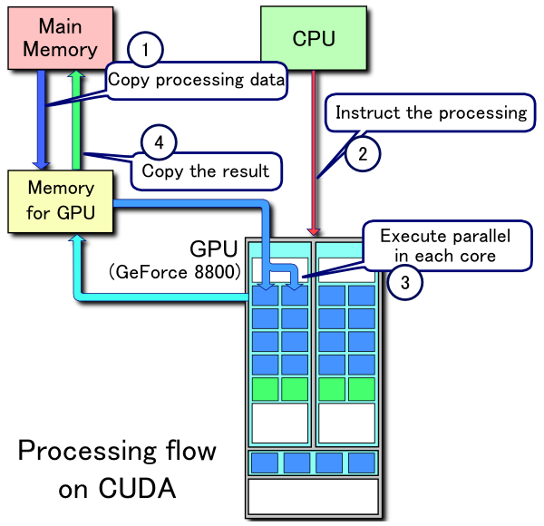
Just like your CPU, your GPU has access to it’s own memory. Programming a GPU entails managing your CPU’s memory along with your GPU’s memory. If you would like your GPU to have access to some memory you’re using on the CPU, you’ll have to allocate memory on the GPU and copy it over.
If you don’t tell the GPU to perform any work, then your CUDA C code is really just C code:
#include <cstdio>
int main() {
  puts("Hello!");
  return 0;
}
You can then invoke NVIDIA’s compiler, NVCC, to compile the program:
$ cat hello.cu
#include <cstdio>
int main() {
  puts("Hello!");
  return 0;
}
$ nvcc hello.cu -o hello && ./hello
Hello!
If you invoke nvcc with the -v flag for extra verbosity, you can see that nvcc actually uses a host compiler to build the parts of your program that don’t involve running code or manipulating memory on the GPU.
nvcc uses multiple passes, where it compiles the CUDA code and generates host-only source for the host compiler to compile.
See this Compiler Explorer link and look at the compilation output window in the bottom right pane to see all the output.
Notice that GCC is invoked, along with the program ptxas.
PTX is an assembly target, so your CUDA programs will emit ptx code which can be run on your GPU’s special purpose processing units.
The command line flags for code generation can be complicated.
Refer to the official CUDA programming guide when needed.
Just as you can use asm volitile("" : : : ""); in C and C++ to write inline assembly, you can also write inline ptx assembly in your programs.
Also like C and C++, it is almost certainly more effective for you to write your code in a higher level language like CUDA C++, and write PTX after profiling and testing, when you are sure you need it.
If you’re careful, you might also have noticed that GCC was passed the command line argument -x c++, even though we’re working in plain CUDA C.
This is because cuda code is by default built on the host as C++.
If you use the oldest CUDA compiler available on Compiler Explorer, you’ll see that it still defaults to building the host code under C++14.
The full NVCC compilation pipeline is depicted below:

Using the CUDA Runtime
In this example, we introduce three aspects of the CUDA programming model:
- The special keyword
__global__ - Device memory management
- Kernel launches
// square.cu
#include <cstdio>
#include <cuda.h>
#include <cuda_runtime.h>

__global__ void square(int *ar, int n) {
  int tid = threadIdx.x;
  if (tid < n)
    ar[tid] = ar[tid] * ar[tid];
}

int main() {
  #define N 10

  // Allocate static memory on host
  int ar[N];
  for (int i=0; i < N; i++) ar[i] = i;

  // Allocate memory on device, copy from host to device
  int* d_ar;
  cudaMalloc(&d_ar, sizeof(int[N]));
  cudaMemcpy(d_ar, ar, sizeof(int[N]), cudaMemcpyHostToDevice);

  // Launch kernel to run on the device
  square<<<1, 15>>>(d_ar, N);

  // Copy memory back from device
  cudaMemcpy(ar, d_ar, sizeof(int[N]), cudaMemcpyDeviceToHost);

  // Display values after kernel
  for (int i=0; i < N; i++)
    printf("%d ", ar[i]);
  puts("");

  // Deallocate memory
  cudaFree(d_ar);
  return 0;
}
$ nvcc square.cu -o square
$ ./square
0 1 4 9 16 25 36 49 64 81
__global__ indicates that the code runs on the device and is called from the host.
Keep in mind that we have two memory spaces and two execution spaces.
The following table enumerates common operations in C along with their CUDA counterpart:
| Operation | C | CUDA | Notes |
|---|---|---|---|
| Dynamically allocate memory | malloc |
cudaMalloc |
|
| Copy memory from one location to another | memcpy |
cudaMemcpy |
|
| Deallocate memory | free |
cudaFree |
|
| Call function | func() |
func<<<gridSize, blockSize, sharedMemSize, cudaStream>>>() |
Triple angle-brackets indicate you are running in the device execution space |
The kernel launch parameters determine how many streaming multiprocessors (SMs) will execute code on the GPU.
The first two parameters are objects of type dim3, and they can be up to three-dimensional vectors.
The first kernel launch parameter is the grid size, and the second is the block size.
Grids consist of blocks.
Blocks consist of threads.
Therefore, the total number of threads launched by your kernel will be:
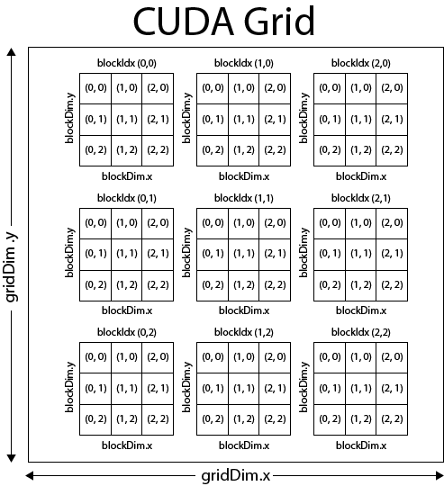
CUDA kernels may be launched with a 1-3 dimensional grid, and a 1-3 dimensional block. The image below might have been launched with these kernel launch parameters:
  dim3 grid_size(3, 3, 1);
  dim3 block_size(3, 3, 1);
  myfunc<<<grid_size, block_size>>>();
You might also notice that we guard our operation with this if statement.
  if (tid < n)
    ar[tid] = ar[tid] * ar[tid];
For performance reasons, it’s usually best to launch your kernels with a multiple of the number of threads in a given block on your GPU, so you may launch with more GPU threads than you need.
Shared Memory
Although each thread launches with its own stack memory, threads can share memory just like OS threads. The third kernel launch parameter determines how many bytes will be allocated for each block that is launched.
#include <cstdio>
#include <cuda.h>
#include <cuda_runtime.h>

__global__ void mulsum(int* a, int* b, int* out, int n) {
  int tid = threadIdx.x;
  extern __shared__ int tmp[];
  /* ▲
   * │  ┌───────────────────────────────┐
   * │  │External and shared, allocated │
   * └──┤by the cuda runtime when kernel│
   *    │         is launched           │
   *    └───────────────────────────────┘
   */
  if (tid >= n)
    return;

  tmp[tid] = a[tid] * b[tid];

  __syncthreads();

  if (tid == 0) {
    int sum = 0;
    for (int i=0; i < n; i++)
      sum += tmp[i];
    *out = sum;
  }
}

int main() {
  #define N 10

  int a[N];
  for (int i=0; i < N; i++) a[i] = i;

  int b[N];
  for (int i=0; i < N; i++) b[i] = i;

  int* d_a;
  cudaMalloc(&d_a, sizeof(int[N]));
  cudaMemcpy(d_a, a, sizeof(int[N]), cudaMemcpyHostToDevice);

  int* d_b;
  cudaMalloc(&d_b, sizeof(int[N]));
  cudaMemcpy(d_b, b, sizeof(int[N]), cudaMemcpyHostToDevice);

  int* d_out;
  cudaMalloc(&d_out, sizeof(int));

  mulsum<<<1, N, sizeof(int[N])>>>(d_a, d_b, d_out, N);
  /*             ▲
   *             │
   *    ┌────────┴────────────────────────────┐
   *    │Size of shared memory to be allocated│
   *    │         for kernel launch           │
   *    └─────────────────────────────────────┘
   */

  int out;
  cudaMemcpy(&out, d_out, sizeof(int), cudaMemcpyDeviceToHost);
  printf("%d\n", out);

  cudaFree(d_a);
  cudaFree(d_b);
  cudaFree(d_out);
  return 0;
}
$ nvcc mul-sum-reduce.cu && ./a.out
285
Notice how our shared memory is declared:
extern __shared__ int tmp[];
It is external because we are not allocating the memory in our kernel; it’s allocated by the cuda runtime when we pass the third parameter to the kernel launch parameters:
mulsum<<<1, N, sizeof(int)*N>>>(d_a, d_b, d_out, N);
               ▲
               │
 ┌─────────────┴───────────────────────┐
 │Size of shared memory to be allocated│
 │         for kernel launch           │
 └─────────────────────────────────────┘
There can only be one segment of shared memory in a kernel launch, so the shared memory segment will be interpreted as whatever type we declare our shared memory with.
In this case, it’s an array of ints.
Although there is strictly one segment of shared memory in a kernel launch, you can still declare multiple variables as __shared__, so long as they all fit in the allocated shared memroy.
We also introduced another CUDA extension to the host language: __syncthreads().
__syncthreads() is a fence or barrier, a point which no thread in that block can cross until all threads have reached it.
__syncthreads()
There are many other CUDA primitives for atomic, and synchronization operations, such as atomicAdd.
CUDA Mat-Vec Multiply
We again return to our matvecmul example, this time armed with some knowledge about the CUDA runtime and some software and hardware abstractions.
#include <cstdio>
#include <cuda.h>
#include <cuda_runtime.h>

__global__ void matvecmul(int* mat, int* vec, int* outv,
                          int m, int n) {

  int rowidx = blockIdx.x;
  int colidx = threadIdx.x;

  extern __shared__ int tmp[];

  if (colidx < n && rowidx < m) {
    tmp[colidx] = mat[colidx + (rowidx * n)] * vec[colidx];

    __syncthreads();

    if (colidx == 0) {
      int sum = 0;
      for (int i=0; i < n; i++)
        sum += tmp[i];
      outv[rowidx] = sum;
    }
  }
}

int main() {
  #define M 10
  #define N 15

  int a[M*N];
  for (int i=0; i < M*N; i++) a[i] = i;

  int b[N];
  for (int i=0; i < N; i++) b[i] = i;

  int* d_a;
  cudaMalloc(&d_a, sizeof(int[M*N]));
  cudaMemcpy(d_a, a, sizeof(int[M*N]), cudaMemcpyHostToDevice);

  int* d_b;
  cudaMalloc(&d_b, sizeof(int[N]));
  cudaMemcpy(d_b, b, sizeof(int[N]), cudaMemcpyHostToDevice);

  int* d_c;
  cudaMalloc(&d_c, sizeof(int[M]));

  matvecmul<<<M, N, sizeof(int[N])>>>(d_a, d_b, d_c, M, N);

  int c[M];
  cudaMemcpy(c, d_c, sizeof(int[M]), cudaMemcpyDeviceToHost);

  cudaFree(d_a);
  cudaFree(d_b);
  cudaFree(d_c);
  return 0;
}
After adding some printing code to our example above, we get the following:
$ nvcc matvecmul.cu && ./a.out
Matrix:
   0    1    2    3    4    5    6    7    8    9   10   11   12   13   14
  15   16   17   18   19   20   21   22   23   24   25   26   27   28   29
  30   31   32   33   34   35   36   37   38   39   40   41   42   43   44
  45   46   47   48   49   50   51   52   53   54   55   56   57   58   59
  60   61   62   63   64   65   66   67   68   69   70   71   72   73   74
  75   76   77   78   79   80   81   82   83   84   85   86   87   88   89
  90   91   92   93   94   95   96   97   98   99  100  101  102  103  104
 105  106  107  108  109  110  111  112  113  114  115  116  117  118  119
 120  121  122  123  124  125  126  127  128  129  130  131  132  133  134
 135  136  137  138  139  140  141  142  143  144  145  146  147  148  149

Vector:
   0    1    2    3    4    5    6    7    8    9   10   11   12   13   14

Output:
1015 2590 4165 5740 7315 8890 10465 12040 13615 15190
This BQN example verifies the output from our CUDA program:
   Mul ← +˝∘×⎉1‿∞
   m←10‿15⥊↕200
   v←↕15
   m Mul v
⟨ 1015 2590 4165 5740 7315 8890 10465 12040 13615 15190 ⟩
In our CUDA C example, we launch a block for each row of our matrix. This way, we can share memory between each thread operating on a given row of the matrix. A single thread per row can then perform the sum reduction and assign the value to the index in the output vector.
CUDA C++
Naive Approach
In our previous CUDA C example, we weren’t really using CUDA C perse, but CUDA C++. If you read the introductory chapter in the official NVIDIA CUDA Programming guide, you’ll see that CUDA C is really just CUDA mixed with the common language subset between C and C++ on the host. We were using CUDA C++ the whole time, we just restricted ourselves to the C subset of C++ for simplicity.
#include <cstdio>
#include <thrust/device_vector.h>
#include <thrust/host_vector.h>
#include <thrust/sequence.h>
#include <cuda.h>
#include <cuda_runtime.h>

/* ┌───────────────────────────┐
   │Using thrust's pointer type│
   │     instead of int*       │
   └───────────────────────────┘ */
__global__ void matvecmul(
    thrust::device_ptr<int> mat,
    thrust::device_ptr<int> vec,
    thrust::device_ptr<int> outv,
    int m, int n) {

  int rowidx = blockIdx.x;
  int colidx = threadIdx.x;

  extern __shared__ int tmp[];

  if (colidx < n && rowidx < m)
  {
    tmp[colidx] = mat[colidx + (rowidx * n)] * vec[colidx];

    __syncthreads();

    if (colidx == 0) {
      int sum = 0;
      for (int i=0; i < n; i++)
        sum += tmp[i];
      outv[rowidx] = sum;
    }
  }
}

int main() {
  #define M 10
  #define N 15

  /* ┌────────────────────────────────┐
     │ Using thrust's host and device │
     │    vectors over raw arrays.    │
     │No longer need to use cudaMemcpy│
     │        or cudaMalloc!          │
     └────────────────────────────────┘ */
  thrust::device_vector<int> a(M*N);
  thrust::sequence(a.begin(), a.end(), 0);

  thrust::device_vector<int> b(N);
  thrust::sequence(b.begin(), b.end(), 0);

  thrust::device_vector<int> c(M, 0);

  matvecmul<<<M, N, sizeof(int[N])>>>(a.data(), b.data(), c.data(), M, N);

  /* ┌────────────────────────────┐
     │The assignment operator will│
     │   perform the cudaMemcpy   │
     └────────────────────────────┘ */
  thrust::host_vector<int> out = c;

  puts("Output:");
  for (int i=0; i < M; i++)
    printf("%d ", out[i]);
  puts("");
  return 0;
}
$ nvcc thrust-ex.cu && ./a.out
Output:
1015 2590 4165 5740 7315 8890 10465 12040 13615 15190
As you can see, the code looks quite similar, except for the lack of memory management. This is hiding a few extra details as well. In our original CUDA example, we first allocate and assign to memory on the host before copying it to the device. In this example, we allocate memory on the device first, and perform assignments on the device.
In this line, we allocate device memory for our matrix, and assign values to it on the device.
  thrust::device_vector<int> a(M*N);
  thrust::sequence(a.begin(), a.end(), 0);
thrust::sequence is almost identical to std::iota or for (int i=0; i < N; i++) vec[i] = i;, except that it may execute on the device.
In this new example, we launch three kernels instead of one: one for each call to thrust::sequence, and one for our manual kernel launch.
You can look at the details of the ptx assembly in Compiler Explorer here.
More Sophisticated Approach
Remember all that fuss about fundamental algorithms in the earlier sections? How our fundamental algorithm here is a transform-reduce?
Well, in our first-pass CUDA implementation, we don’t really use this to our advantage. Our kernel contains the following lines:
    if (colidx == 0) {
      int sum = 0;
      for (int i=0; i < n; i++)
        sum += tmp[i];
      outv[rowidx] = sum;
    }
While we used a raw loop at least once per block, an optimized reduction will perform something like the following:

Extremely performant reductions are actually quite hard to get right - it’s easy to get some parallelism in a reduction, but it takes significant effort to truly maximize the speed you can get from a GPU. This slidedeck from the NVIDIA developer blog details various approaches to optimizing a reduction operation on a GPU. Thrust’s reduce implementation will even select different strategies and launch parameters based on the sizes of the data it operates on.
The point of this Thrust discussion is not to dissuade you from writing raw CUDA kernels - it’s to dissuage you from doing it too early. In the majority of cases, it’s likely that using a library around raw CUDA kernels will result in faster code and less development time. Once you have already written your code using known algorithms, once you have tested your code to demonstrate its correctness, once you have profiled your code to demonstrate where the performance bottlenecks are on the target architectures you care about, then it makes sense to write raw CUDA kernels.
Use sane defaults, only optimize after profiling and testing
So let’s try again, using Thrust’s parallel algorithms to compute the reductions for each row of the matrix-vector multiplication (godbolt link here):
#include <cstdio>
#include <thrust/iterator/zip_iterator.h>
#include <thrust/tuple.h>
#include <thrust/device_vector.h>
#include <thrust/host_vector.h>
#include <thrust/sequence.h>

__global__
void broadcast_to_matrix(thrust::device_ptr<int> mat,
    thrust::device_ptr<int> vec,
    int m, int n) {
  const auto col = blockIdx.x;
  const auto row = threadIdx.x;

  if (row < m and col < n)
    mat[col+(row*n)] = vec[col];
}

int main() {
  #define M 10
  #define N 15

  thrust::device_vector<int> a(M*N);
  thrust::sequence(a.begin(), a.end(), 0);

  thrust::device_vector<int> b(N);
  thrust::sequence(b.begin(), b.end(), 0);

  thrust::device_vector<int> broadcasted_b(M*N);
  broadcast_to_matrix<<<N, M>>>(broadcasted_b.data(), b.data(), M, N);

  thrust::host_vector<int> c(M);

  thrust::zip_iterator iter(thrust::make_tuple(a.begin(), broadcasted_b.begin()));

  for (int i=0; i < M; i++)
    c[i] = thrust::transform_reduce(iter+(i*N), iter+(i*N)+N,
        [] __device__ (auto tup) -> int {
          return thrust::get<0>(tup) * thrust::get<1>(tup);
        },
        0,
        thrust::plus<int>()
        );

  puts("Output:");
  for (int i=0; i < M; i++)
    printf("%d ", c[i]);
  puts("");
  return 0;
}
Since we’re using some more fancy C++ features, we have to pass some extra flags to the compiler:
$ nvcc -std=c++17 --extended-lambda fancy.cu && ./a.out
Output:
1015 2590 4165 5740 7315 8890 10465 12040 13615 15190
The first kernel is launched manually, since we’re just broadcasting values from the vector to another vector to match the shape of our matrix. We perform this step so we can create a zip iterator from the matrix and the broadcasted vector:
thrust::zip_iterator iter(thrust::make_tuple(a.begin(), broadcasted_b.begin()));
This means we can feed the single iterator into our transform_reduce operation.
Elements obtained by the zip iterator are passed into our lambda function, and we simply multiply the two values together, before using the plus functor to reduce the vector of intermediate values for a given row into a scalar:
  for (int i=0; i < M; i++)
    c[i] = thrust::transform_reduce(iter+(i*N), iter+(i*N)+N,
        [] __device__ (auto tup) -> int {
          return thrust::get<0>(tup) * thrust::get<1>(tup);
        },
        0,
        thrust::plus<int>()
        );
If we want to use threading on the host as well, we can even use an OpenMP directive:
#pragma openmp parallel for
  for (int i=0; i < M; i++)
    c[i] = thrust::transform_reduce(iter+(i*N), iter+(i*N)+N,
        [] __device__ (auto tup) -> int {
          return thrust::get<0>(tup) * thrust::get<1>(tup);
        },
        0,
        thrust::plus<int>()
        );
We’ll have to tell nvcc to pass the -fopenmp flag to the host compiler:
$ nvcc -std=c++17 --extended-lambda -Xcompiler -fopenmp fancy.cu
The Best Tool for the Job
We have by now hopefully learned that we should use the most specialized tool for the job, and we should write kernels by hand only when we’re sure we can do better than your libraries of choice. We can take this principle one step further with a little extra knowledge of our problem.
A matrix-vector product is a very common linear algebra operation, and a member of the Basic Linear Algebra Subroutines interface, which CUDA provides a library for (CUBLAS). Because this is such a common operation, NVIDIA provides an extremely fast implementation - far more optimized than anything we would write by hand.
This knowledge of our problem leads us to using the most appropriate library, and likely to the fastest solution.
#include <cstdio>
#include <thrust/device_vector.h>
#include <thrust/host_vector.h>
#include <thrust/sequence.h>
#include <cuda.h>
#include <cuda_runtime.h>
#include <cublas_v2.h>

int main() {
  #define M 10
  #define N 15

  cublasHandle_t ch;
  cublasCreate(&ch);

  thrust::device_vector<double> a(M*N);
  thrust::sequence(a.begin(), a.end(), 0);

  const double alpha = 1.0;
  const double beta = 0.0;

  thrust::device_vector<double> b(N);
  thrust::sequence(b.begin(), b.end(), 0);

  thrust::device_vector<double> c(M);

  #define PTR(x) thrust::raw_pointer_cast(x.data())
  cublasDgemv(
      ch,
      CUBLAS_OP_T,
      N, M,
      &alpha,
      PTR(a), N,
      PTR(b), 1,
      &beta,
      PTR(c), 1
      );
  #undef PTR

  thrust::host_vector<double> hc = c;

  puts("Output:");
  for (int i=0; i < M; i++)
    printf("%.1f ", hc[i]);
  puts("");

  cublasDestroy(ch);

  return 0;
}
$ nvcc cublas.cu -lcublas && ./a.out
Output:
1015.0 2590.0 4165.0 5740.0 7315.0 8890.0 10465.0 12040.0 13615.0 15190.0
Conclusion
BQN Example
Personally, I use BQN to prototype solutions to problems and to better understand the fundamental algorithms at play; you don’t have to know an APL in order to understand this, but it might be helpful. Feel free to skip this section; it is not critical to understanding the concepts.
Here’s a permalink to the BQN snippet.
   # Same matrix as in our C example
   mat ← 3‿3⥊↕10
┌─
╵ 0 1 2
  3 4 5
  6 7 8
        ┘
   # Same vector as in our C example
   vec ← 3⥊2
⟨ 2 2 2 ⟩

   +˝⎉1 mat×vec
⟨ 6 24 42 ⟩
The core algorithm is seen in the final expression:
+˝⎉1 mat×vec
▲    ▲
│    │     ┌───────────────────────────┐
│    └─────┤Multiply rows of mat by vec│
│          │        element-wise       │
│          └───────────────────────────┘
│     ┌─────────────────────────┐
│     │Sum-reduce rows of matrix│
└─────┤ resulting from mat×vec  │
      └─────────────────────────┘
Alternatively:

Links, References, Additional Reading
- BQN matvecmul example
- Matrix-Vector Product image
- UT Austin slides on loop-carried dependencies and parallelism
- How to Write Parallel Programs: A First Course
- Thrust parallel algorithms library
- ADSP podcast episode from the lead HPC architect at NVIDIA discussing speed vs efficiency
- Bryce Adelstein Lelbach’s talk on C++ standard parallelism
- Kokkos
mdspansingle header - CUDA C Introduction Slides
- More sophisticated CUDA matrix-vector product implementations
- Slides on CUDA reduction operation